Yesterday I listened to a talk by
Victor Yakovenko of the University of Maryland about the physics of money and it was quite interesting. I think that after this talk I am finally beginning to understand economics while at the same time I suspect that most economists don't.
In his talk he said that back in 2000 he published
a paper on how to apply statistical mechanics to free market economics. He did it as a hobby and did not consider it to be very important, meaning he still did his normal research involving condensed matter physics. A few years later he realized that his paper on the statistical mechanics of money was getting more citations than any of his other papers, so he switched his focus of research to
Econophysics.
One of the most interesting results that he found was that in a free (random) system of monetary exchanges the natural distribution of money will converge, over time, on a
Boltzmann-Gibbs distribution. The argument is simple. In stat mech you have a system where small, discreet amounts of energy are passed from one particle to another. This system leads to a probability distribution characterized by the equation [all images come from
Dr. Yakovenko unless otherwise stated]:
Where we have the probability of finding a particle at a particular energy level on the left and the energy, represented by ε, and temperature on the right. If we change the energy to money (or income) and temperature to average income we have:
So what does this mean in reality? Well consider a system where everyone is given $10 to start out and they can engage in economic transactions worth $1 each (they can either pay $1 or receive $1 per transaction), with the requirement that if anyone reaches $0 they can no longer pay money (i.e. they can't go into debt) but they can receive money, it's just that the other person does not receive money in return (think of it as work done). Over time this system moves to maximum entropy and achieves a Boltzmann-Gibbs distribution. An undergrad at Caltech named Justin Chen, who worked with Dr. Yakovenko, made an animation of this system [you can find more information on this animation
here]:
As we see, the system starts out as a delta function but changes to a Gaussian distribution, but because of the hard boundary at m=0 (think of it as the ground state) we end up with a Boltzmann distribution. So as soon as they thought about this they started to look into other things, such as allowing for debt, taxes, and interest on the debt (this is of course assuming conservation of money). When they allowed for debt, but only down to a certain level (i.e. the ground state was shifted to a negative value), they found that it did not change the shape of the distribution but it did raise the temperature of the money (raised the average money).

The way this works is that every time someone goes into debt (negative money) an equivalent amount of positive money is created. Thus while the total amount of money has not changed, the amount of positive money goes up, raising the temperature and thus creating the illusion that there is more money. While this does put some people into debt, it does raise the number of people with more money, thus it makes more people rich (note: the rich do get richer under this system, but the main effect is that there are more rich people. So it is not just that the same people get richer because of the debt, it's that more people have more money). But you may say that this is not very physical because in the real world there is no low limit of debt. In theory someone could have infinite debt (infinite in the sense of very, very large). And in their models, if they remove the debt floor they have precisely this effect, the number of people who go into deep debt grows until we have a flat line fore the distribution.
This problem was solved in 2005 by
Xi, Ding and Wang when they considered the effect of the
Required Reserve Ratio (RRR), which to explain simply limits the amount of money that lenders can lend. In terms of the simulations this means that every time someone goes into debt the corresponding positive money that is created cannot all be used to finance more debt. A certain amount must be held in reserve. This limits the total debt that can be issued by the system based on the total amount of money that was in the system to begin with. The end effect is that the distribution becomes something like this [From Xi, Ding and Wang]:

This effectively creates a double exponential distribution that is centered about the average money amount. Now we can start to look at some of the effects that things like taxes and interest have on this system. First, interest. If we add interest the system does not have a stable state and without any form of check the system will expand to infinity, in both directions. Second, taxes. Assuming a tax on all transactions, either a fixed amount or a percentage, and then assuming the tax is then evenly redistributed, this will shift the peak slightly to the right, though it will not change the edges that much. So a redistributive tax will raise the income of people near 0 slightly, away from 0, but it will have very little effect on the overall shape or the edges (the very rich or the most indebted). If we allow for bankruptcies then that acts as a stabilizing force on the system, that is, it keeps it from spreading to infinity. Thus interest creates no stationary state, but bankruptcy creates a stable state. He noted that what the Fed is currently doing is in response to the economic crisis, the negative end of the money (the debt) has shrunk considerably because of foreclosures, and other problems, but to keep the positive end from shrinking as well they pumped more money into the system to maintain the size and shape of the distribution. While this does prevent the positive side from collapsing, the trade off is that there is more money put into the system, creating the potential of inflation. (As a side note: part of the reason we got into this mess in the first place is because banks found a way around the RRR requirement, allowing them to issue more debt than they should have, which gave the impression that the economy was booming because there was more positive money, but this ignored the fact that there was a corresponding amount of debt being created. The debt was limited by personal bankruptcy and thus created a domino effect that removed both the debt, but also a significant amount of the positive money. We have yet to even come close to recovering to the level we were at before. If you hear talk about the Fed keeping interest rates low to spur lending, they are trying to create more positive money through lending, by creating negative money, but because that is not working they have begun printing more money (buying government bonds) to create more positive money without having to create more negative money.)
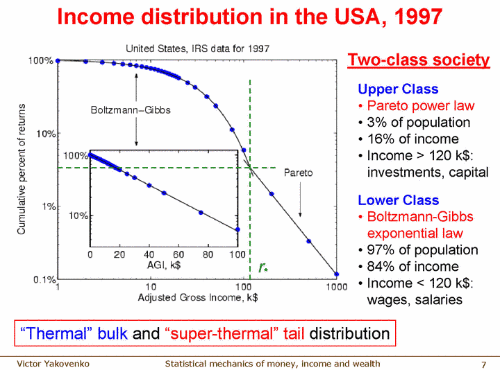
Now let's look at some real data. Using US census data from 1996 they plotted income and found that it fits nicely to a Boltzmann distribution, as long at you do not get too close to $0 (above $10,000 works fine).
But this only works up to a point. They found that up to some point the income of people fits very nicely to a Boltzmann Distribution but above a certain point income behaves differently. If you plot all they way up into the highest levels of income you see a clear point where the income changes from Boltzmann-Gibbs to a
Pareto power law distribution.
They noted that while the lower Boltzmann distribution does not change much over the years, despite recessions and boom times, the top "super-thermal" tail changes a lot depending on the economy. This super-thermal tail represents only 3% of the people, but holds anywhere between 10-20% of the money. The total amount of the inequality depends on the economy at the time.
So what happens when this distribution gets upset by programs such as social welfare or other effects. In a
paper published in 2006, Banerjee, Yakovenko, and Di Matteo give the following graph showing the distribution of income in Australia.
The spike on the lower end is the welfare limit. People below this limit are brought up to the limit though welfare, but people just above it are also brought down to the level because of taxes. Hence the spike but also the dips on both sides. The result is more equality, but at the expense of lowering the entropy of the system and creating this deviation from the normal distribution. The desirability of doing something like this is debatable (as one professor asked after the talk, "What's wrong with inequality?")
When asked about the predictive power of this his response was, "None." He explained that this data takes a long time to collect and to analyze, which creates a lag of several years in the data. But by the time the data has been collected and analyzed and we are able to see a bubble (like the housing bubble) the bubble has already burst and we have moved on. But this also means that modern free market economics behaves in a very statistical manner and can thus be controlled (in theory), which is what the Fed is currently trying to do. Dr. Yakovenko did not get too much into the politics of it, but he did make it clear that he did not agree with the way the bailouts were handled, and the current tactic of the Fed. But it was also clear that he preferred a free market, though a heavily regulated one. He was also very concerned about the inequality in the system, and noted the existence of two classes of people and made reference to Karl Marx at that point.
On the whole I was rather impressed with what he was doing and like I said, I think I am finally beginning to understand economics. Someone just had to explain it to me in terms of physics and it made perfect sense.
XI, N., DING, N., & WANG, Y. (2005). How required reserve ratio affects distribution and velocity of money☆ Physica A: Statistical Mechanics and its Applications, 357 (3-4), 543-555 DOI: 10.1016/j.physa.2005.04.014