Testing the ∇⋅ B = 0 condition in numeric solvers

When considering magnetic fields in computer simulations using the equations of magnetohydrodynamics (MHD) we have to take into account one of Maxwell's equations, namely:

∇⋅ B = 0

This is the condition that there is no divergence in the magnetic field, which in physical terms means that there are no magnetic charges. That is, we don't have particles floating about that create magnetic field lines. All of the magnetic flux that enters a given volume must leave the volume.

Mathematically this is usually straight forward (well sort of, except for those that have had to suffer through Jackson), but when it comes to computer simulations it turns out that this condition is very hard to preserve. There are several different methods used to preserve this condition and for those that are interested there is an excellent paper by Gábor Tóth that describes many of these methods (Gábor Tóth, Journal of Computational Physics, 161, 2, 2000, Pages 605-652).

While I am not going to discuss how these methods work, I will note that they are all imperfect. Because of the fundamental way simulations and computers work, there will always be some error, which means the divergence condition will never be met. The way of dealing with this usually involves making the error from the numerical solver to be as small as possible. While some ways of solving the MHD equations can make the error very small, it comes at the cost of making the code run slower (for example the projection method may be better than other methods in almost all situations, but it comes at the cost of a 20% increase in the time needed compared to the base method for they hydro equations. For reference, of the seven methods investigated by Tóth the next slowest only added 7% to the time).

But the question is, how do we test the accuracy of these different methods. Well, the easiest way is to have them solve a problem that we already know the answer for analytically and then see how well the code does at getting the correct answer. While many codes will do well with a simple problem, the idea is to get a very difficult problem and see how the code handles it.

One such problem is the Smooth Alfvén Wave test. This test takes a polarized magnetic field and has it propagate across the grid. Using this special set up it will create standing Alfvén waves. Because of the nature of the Alfvén waves and how they interact with the material, for this particular test the density should not change and the wave should not dissipate. That is, after one period the entire system should return to its original state. Any change in the density, energy, velocity or magnetic field is an indication of the errors introduced by the numeric solver. By knowing the initial conditions we can then calculate the change and therefore the error.

So in a real simulation, what would this look like? Well something like this:

This is a video of the Smooth Alfvén Wave test, with a circularly polarized magnetic field. This is a 2D simulation (well, 2.5D but anyway...) with a constant density slab of material with constant pressure. The wave propagates from the top right corner towards the bottom left. The color of the slab indicates the density. The initial density is a grey color and thus any other color you see in the slab indicates an error in the solver (there is a color legend in the video). The arrows indicate the velocity (and the color of the arrows does not mean anything, I just made them pink so that you could see them). The velocity points in the same direction as the magnetic field, so the arrows also show magnetic field. The test runs for five periods.

As I mentioned, any color, red or blue, you see in the slab indicates a numerical error, but while it make look like this was a bad simulation, note that the difference is only 4.3 e -4. This is still small and acceptable for most applications. If I ran it for longer, the errors would grow. If I started adding in other things, again the error would grow. In this case I can compare the result to the analytic solution, but in the case where there is no analytic solution we have to rely of either proven methods, better resolution or in the worst case, just assume that the errors are small (shudder).

This simulation was run in Athena, which uses a constrained transport method to address the ∇⋅ B = 0 problem, and it took about 3 minutes to run on my laptop. I rendered it in Paraview, which after taking a few minutes to set it up, it only took 2 or 3 minuets to render.

Non-uniformity necessary for longevity

Recently I have been looking at a series of papers detailing some hydrodynamic simulations performed by a research group in Australia (incidentally they are using a modification of a hydro code called VH-1 originally written by John Blondin at NC State University, just down the road from me. Think U of U and BYU, complete with similar colors, only BYU has dark blue and UNC has light blue. Anyway back to my post...). In their second paper the group finds "that the ability of the cloud to radiate heat is crucial for its survival", and that a non-uniform cloud will survive longer than a uniform cloud when hit by an expanding shockwave.

Now for a brief rundown of their research: After combining the hydro code VH-1 with a thermal cooling code called MAPPINGS III they ran their simulations of uniform spherical clouds and non-uniform fractal clouds. They introduced a shockwave that would accelerate and fragment the cloud (the shockwave would come from a supernova or an AGN). The motivation was to find out how filamentary structures are formed as observed in the center of galaxies such as NGC 3079 (picture credit to my adviser):

[Close up of the center]

These bright H-alpha regions are somewhat of a mystery as to how they form exactly. And the purpose of the simulations was to find out how they formed and what they look like in 3D. Part of the problem is that if you introduce a strong interstellar wind, such as from an AGN or a series of supernovas then according to previous simulations, the clouds of dense interstellar gas would not survive long enough to for structures like this. So this group in Australia tried performing the simulations, but included thermal cooling and shocked non-uniform clouds. When they did this they found that even though the non-uniform clouds will fragment faster than the uniform (spherical) clouds, the effect of thermal cooling causes the fragments to live longer than the larger uniform cloud. This allows a cloud to survive long enough to form filaments such as the ones observed above.

If you think about it, what is going on here is that when both the uniform and non-uniform clouds are shocked they will both heat up and begin radiating away heat. But the non-uniform clouds, due to their inherent instabilities will fragment into many smaller clouds thus increasing the surface area to volume ratio. Because the amount of heat stored by a cloud depends on its volume but the rate of heat loss depends on the surface area, if you keep the cloud together (i.e. uniform) then when it heats up it will not radiate as efficiently as the cloud with more surface area. Hence why car radiators and other similar devices have cooling fins.

If you had asked most people to predict which cloud would last longer, the dense, spherical cloud or the sparse, non-uniform cloud, most would probably say the denser cloud, but it turns out that the non-uniform cloud would last longer because of the non-intuitive concept of radiative cooling.

Spots in Southern California, Part 3

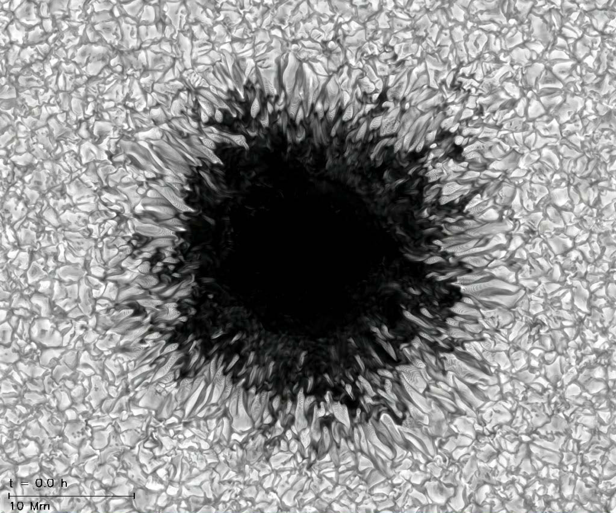
How do you build a sun spot?  Previously one needed a sun, which is very inconvenient in terms of logistics and safety issues.  It turns out that now you can build one with just an amazing computer code and a large supercomputer, which is much more convenient and it runs out pretty darn effective.  Below are a real and a simulation sunspot.  I'll let you figure out which is which.

In a truly groundbreaking simulation, Matthias Rempel of the National Center for Atmospheric Research here in Boulder has created a realistic simulation of a sunspot that appears to correctly reproduce almost all of a the observed features of real sunspots.

This is the kind of numerical model most of us computational scientists dream about at night.

A quick shot of my galaxy simulation

[Updated]

I mentioned previously that I have been working on a galaxy simulation with a star forming region in the center. Things have been progressing, I think I can go to running 3D simulations sometime in the next two months. I will share more information when I have it, but I just wanted to share a cool picture that I made from my simulation.This is a density map of the r and z directions (x and y, on this image) of a galaxy, or a slice in the x-z plane at y=0 if you prefer. So top and bottom of the image correspond to above and below the galaxy. We are looking at the galactic disk edge on.

There are a few cool things about this image that made me excited, mostly the long filaments coming out of the galaxy. I was excited about this because that is almost exactly what we see in real galaxies, and is exactly what we are trying to find through simulations. The one problem I had here is I messed up with a certain parameter which made the galaxy not be in hydro-static equilibrium to start out, which means it kind of collapsed in on itself. That explains why the disk is so narrow and so dense.

[Update]
I failed to mention that this image was rendered in ParaView. I also have a few movies that I made relating to this simulation (again rendered in ParaView). A movie showing density can be found here (Note: It is large, 27 MB). Another showing speed (magnitude of velocity) can be found here (also large, 33 MB).